Setting Priors

The prior distribution has many roles in Bayesian inference. Primarily it is used to encode domain knowledge into the model, such as encoding that a parameter must be passive etc. In practice it also becomes a means of stabilizing inferences in complex, high-dimensional problems.

There is a lot of literature on the choice of prior on should use in statistical models, such as uniform priors, Jeffreys’ priors, reference priors, maximum entropy priors and weakly informative priors. In order to select a good prior on have to take the entire model into account. A simple way of doing this is to see if the constructed model generates sane values when generating from the prior [2017Entrp..19..555G].

Lets do an analysis of how to set the prior for a neural network.

import math

import numpy
import matplotlib

matplotlib.use("Agg")
import matplotlib.pyplot as plt
import torch
from torch.nn import init

import borch
from borch import  nn
import borch.distributions as dist
from borch.utils.torch_utils import get_device

DEVICE = get_device()

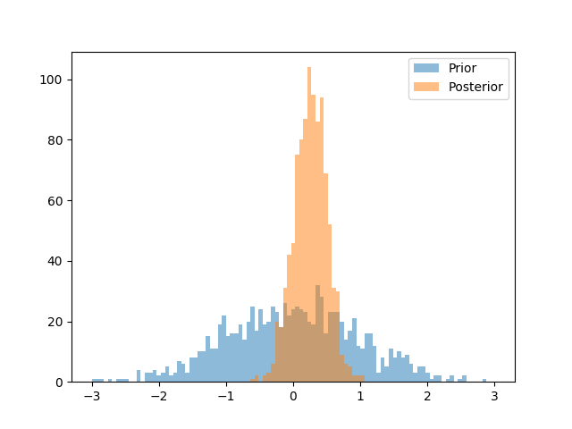
Visualization of prior vs posterior plot

plt.figure()
bins = numpy.linspace(-3, 3, 100)
plt.hist(
    [dist.Normal(0, 1).sample().item() for _ in range(1000)],
    bins,
    alpha=0.5,
    label="Prior",
)
plt.hist(
    [dist.Normal(0.25, 0.25).sample().item() for _ in range(1000)],
    bins,
    alpha=0.5,
    label="Posterior",
)
plt.legend()

Out:

<matplotlib.legend.Legend object at 0x7fa8e326e050>

A very commonly used prior for weights in neural networks is the standard gaussian \(N(0,1)\). In order to set the prior for modules in borch.nn, one has to use the this can be rv_factory argument. To get a standard gaussian one can use the parameter_to_normal_rv as an rv_factory. Lets see how this prior works for a chain of linear layers(for simplicity we negelct non-lineareties between the loinear layes).

In order to see how sane the prior is by sending random noise in an look at the output

net = nn.Sequential(
    nn.Linear(
        1000,
        1000,
        weight=dist.Normal(0, 1),
        bias=dist.Normal(0, 1),
        posterior=borch.posterior.Automatic(),
    ),
    nn.Linear(
        1000,
        1000,
        weight=dist.Normal(0, 1),
        bias=dist.Normal(0, 1),
        posterior=borch.posterior.Automatic(),
    ),
)


borch.sample(net)
out = net(torch.randn(3, 1000, 1000))

lets look at the mean and standard deviation of the out put.

print(out.mean())
print(out.std())

Out:

tensor(0.6967, grad_fn=<MeanBackward0>)
tensor(999.9335, grad_fn=<StdBackward0>)

As we can see the standard deviation is VERY large, unless the target that you are trying to model can be described with that variance, the prior is set wrongly.

Lets see how this prior works for a single linear layer in order to develop some understanding of what is happening

net = nn.Linear(
    1000,
    1000,
    weight=dist.Normal(0, 1),
    bias=dist.Normal(0, 1),
    posterior=borch.posterior.Automatic()
)
borch.sample(net)
out = net(torch.randn(3, 1000, 1000))
print(out.std())

Out:

tensor(31.6465, grad_fn=<StdBackward0>)

Basically one layer increases the standard deviation 30 times, then this will be sent into the next layer creates a compunding effect that makes the standard deviation explode. So in order to avoid this behavior we should construct a prior creates gaussian noise as output from a linear if one feeds it in gaussian noise.

We can get a standarad deviation that is equal to one by calculating the standard deviation of the prior using the method described in “Understanding the difficulty of training deep feedforward neural networks” - Glorot, X. & Bengio, Y. (2010). The std can be used to construct a \(\mathcal{N}(0, \text{std})\) distribution, where

\[\text{std} = \text{gain} \times \sqrt{\frac{2}{\text{fan_in} + \text{fan_out}}}\]

Also known as Glorot initialization.

def xavier_normal_std(shape, gain=1):
    """
    Args:
        shape (tuple): a tuple with ints of shape of the tensor where the xavier init
          method will be used.
        gain (float):  an optional scaling factor

    Returns:
        float, the std to be used in a Gaussian Distribution to achieve a xavier
         initialization.

    """
    tensor = torch.randn(*shape)
    if tensor.ndimension() < 2:
        tensor = tensor.view(*tensor.shape, 1)
    fan_in, fan_out = init._calculate_fan_in_and_fan_out(tensor)
    std = gain * math.sqrt(2.0 / (fan_in + fan_out))
    return std

Lets try the network again with the new prior

net = nn.Sequential(
    nn.Linear(
        1000, 1000, weight=dist.Normal(0, xavier_normal_std((1000, 1000))), posterior=borch.posterior.Automatic()
    ),
    nn.Linear(
        1000, 1000, weight=dist.Normal(0, xavier_normal_std((1000, 1000))), posterior=borch.posterior.Automatic()
    ),
)


borch.sample(net)
out = net(torch.randn(3, 1000, 1000))
print(out.mean())
print(out.std())

Out:

tensor(0.0014, grad_fn=<MeanBackward0>)
tensor(1.0028, grad_fn=<StdBackward0>)

Now we see that the mean is close to zero and the standard deviation is close to one. So form this we can conclude that this is a more sane prior as it generates values in the range that do not explode.

Lets try the same analysis of a single layer for an Conv2d.

net = nn.Conv2d(
    16,
    33,
    (3, 5),
    stride=(2, 1),
    padding=(4, 2),
    dilation=(3, 1),
    weight=dist.Normal(0,1),
    posterior=borch.posterior.Automatic(),
)
borch.sample(net)
out = net(torch.randn(20, 16, 50, 100))
print(out.std())

Out:

tensor(14.8234, grad_fn=<StdBackward0>)

again we see that the standard deviation is to large, lets try setting the prior with the xavier_normal_std.

net = nn.Conv2d(
    16,
    33,
    (3, 5),
    stride=1,
    weight = dist.Normal(0, xavier_normal_std((33, 16, 3, 5))),
    posterior=borch.posterior.Automatic(),
)
borch.sample(net)
out = net(torch.randn(20, 16, 50, 100))
print(out.std())

Out:

tensor(0.8285, grad_fn=<StdBackward0>)

Now we see that we are on the right scale, but we are not at the desired standard deviation of 1 for the output. To address this and also support activation functions we can calculate the standard deviation according to the method described in in “Delving deep into rectifiers: Surpassing human-level performance on ImageNet classification” - He, K. et al. (2015), using a normal distribution. The resulting tensor will have values sampled from \(\mathcal{N}(0, \text{std})\) where

\[\text{std} = \sqrt{\frac{2}{(1 + a^2) \times \text{fan_in}}}\]

Also known as He initialization.

def kaiming_normal_std(shape, a=math.sqrt(5), mode="fan_in", nonlinearity="linear"):
    """
    Args:
        shape (tuple): a tuple with ints of shape of the tensor where
          the xavier init method will be used.
        gain (float):  an optional scaling factor

    Returns:
        float, the std to be used in a Gaussian Distribution to achieve
          a xavier initialization.
    """
    tensor = torch.randn(*shape)
    if tensor.ndimension() < 2:
        tensor = tensor.view(*tensor.shape, 1)
    gain = init.calculate_gain(nonlinearity, a)
    fan = init._calculate_correct_fan(tensor, mode)
    std = gain/ math.sqrt(fan)
    return std


net = nn.Conv2d(
    16,
    33,
    (3, 5),
    stride=1,
    weight=dist.Normal(0, kaiming_normal_std((33, 16, 3, 5))),
    posterior=borch.posterior.Automatic(),
)
borch.sample(net)
out = net(torch.randn(20, 16, 50, 100))
print(out.std())

net = nn.Linear(
    1000, 1000,
    weight=dist.Normal(0, kaiming_normal_std((1000, 1000))),
    posterior=borch.posterior.Automatic()
)
borch.sample(net)
out = net(torch.randn(3, 1000, 1000))
print(out.std())

Out:

tensor(1.0134, grad_fn=<StdBackward0>)
tensor(0.9996, grad_fn=<StdBackward0>)

Now we have constructed a prior that works for both linear and conv layers where we chose to get the stanadard deviation to be close to 1, but this will ofcourse be effected by the activation function on selects. When combining it with activation functions one will have to multiply the std with something approprate depending on the nonlinearity in kaiming_normal_std according to what one have in the network.

Exercises

1. Set up a model to solve CIFAR, where the base model have an accuracy of 80% or higher, then test it with different priors and q_distributions. Test at least two priors discussed above, but also try some other distribution like StudentT.