Hamiltonain Monte Carlo

#
# The `infer` package provides Hamiltonian Monte Carlo (HMC) as a sampling method.
# HMC is an Markov chain Monte Carlo (MCMC) method used to sample from probability
# distributions. We also have support for the No-U-Turn Sampler (NUTS), that is
# an improvement on HMC. Note that both the HMC and NUTS implementations have not
# gone trough rigorous use and is considered experimental.
#
# Let start with the inital imports

import matplotlib
matplotlib.use("Agg")
import matplotlib.pyplot as plt

import borch
from borch import  Module, distributions as dist
from borch.utils.state_dict import add_state_dict_to_state, sample_state
from borch.posterior import PointMass
from borch.infer.model_conversion import model_to_neg_log_prob_closure
from borch.infer.hmc import hmc_step
from borch.infer.nuts import nuts_step, dual_averaging, find_reasonable_epsilon
from borch.utils.torch_utils import detach_tensor_dict

In this example we are going to fit a Gamma and a Normal distribution, where the model is written using borch.

def model(latent):
    latent.weight1 = dist.HalfNormal(.5)
    latent.weight2 = dist.Normal(loc=1, scale=2)

In order to use hmc from alvis.infer, the log_joint should be provided as a closure, i.e. a function or python callable that takes no arguments. The parameters used for hmc also need to be in the unconstraind space, this is easy to do with borch.

trace = PointMass()
latent = borch.Module(posterior=trace)


def model_call():
    borch.sample(latent)
    model(latent)


closure = model_to_neg_log_prob_closure(model_call, latent)

In order to call hmc, parameters needs to be provided as a list, so in order to get them for a borch model one has to run the closure once to get them. hmc_step takes epsilon and L as arguments. epsilon is how big steps the HMC uses when it explores the space and L is the number of leepfrog steps HMC tries to make before it finishes.

state = []
closure()
samples = {}
for i in range(100):
    accept_prob = hmc_step(
        epsilon=.1,
        L=10,
        parameters=trace.parameters(),
        closure=closure
    )
    state = add_state_dict_to_state(latent, state)
    samples[i] = detach_tensor_dict(dict(borch.named_random_variables(latent)))
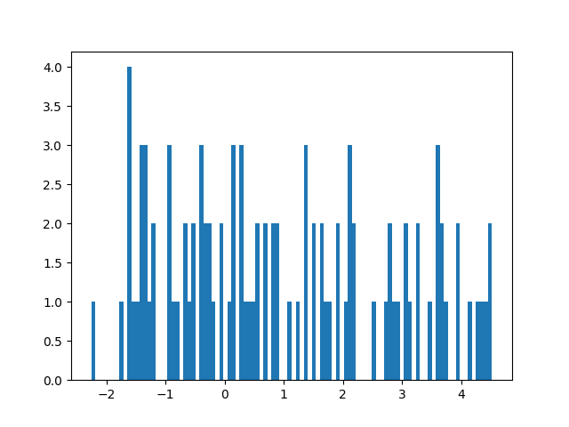
plt.hist([samp['posterior.weight2'] for samp in samples.values()], bins=100)
plt.show()

If one want to restore a current sample such that one can generate from the mode one simply does

for _ in range(1):
    sample_state(latent, state)
    borch.sample(latent)
    pred = model(latent)

In a similar fashion one can use The No-U-Turn Sampler (NUTS) an extension to Hamiltonian Monte Carlo that eliminates the need to set a number of steps leapfrog steps. Empirically, NUTS perform at least as efficiently as and sometimes more efficiently than a well tuned standard HMC method, without requiring user intervention.

Note that the NUTS implementations have not gone trough rigorous use and is considered experimental.

samples_nuts = {}
inital_epsilon, epsilon_bar, h_bar = find_reasonable_epsilon(
                                        trace.parameters(), closure)
epsilon = inital_epsilon
for i in range(1, 100):
    accept_prob = nuts_step(.1, trace.parameters(), closure)
    if i < 25: # the warmup stage
        epsilon, epsilon_bar, h_bar = dual_averaging(accept_prob, i,
                                                inital_epsilon,
                                                epsilon_bar, h_bar)
    else:
        epsilon = epsilon_bar
    samples_nuts[i] = detach_tensor_dict(dict(borch.module.named_random_variables(latent)))
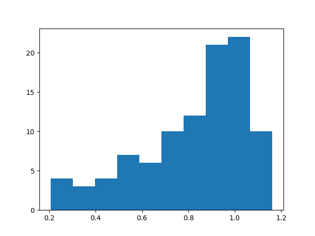
plt.hist([samp['posterior.weight2'] for samp in samples_nuts.values()], bins=10)
plt.show()