Linear Regression

We will have a look at how borch can be used in a simple linear regression setting. We will start off by generating some fake data and construct a model that we will sample from. After that we will try to reconstruct it and see if we can infer the parameters.

Lets start of with importing what we need

import torch
import numpy as np
import matplotlib
matplotlib.use("Agg")
import matplotlib.pyplot as plt

import borch
from borch import infer, distributions as dist

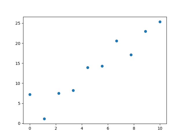
Lets generate some fake data to use

def generate_dataset(n=100):
    x = np.linspace(0, 10, n)
    y = 2*x+4+np.random.normal(0, 2, n)
    return torch.tensor(y, dtype=torch.float32), torch.tensor(x, dtype=torch.float32)

y, x = generate_dataset(10)
plt.scatter(x, y)
plt.show()

We will use borch as a normal PPL to construct a basic linear regression model

def forward(bm, x):
    bm.b = dist.Normal(0, 3)
    bm.a = dist.Normal(0, 3)
    bm.sigma_unconstrained = dist.StudentT(10, 0, 1)
    mu = bm.b * x + bm.a
    # we need sigma to be strictly positive
    sigma = bm.sigma_unconstrained.abs()+0.001
    bm.y = dist.Normal(mu, sigma)
    return bm.y, mu

One can also express the model in line with how torch.nn does it

class Model(borch.Module):
    def __init__(self):
        # a and b will infer the parameters of the distribution.
        self.b = dist.Normal(0, 3)
        self.a = dist.Normal(0, 3)
        # Sigma will infer the width of the noise of the distribution of our data.
        self.sigma = dist.HalfNormal(1)

    def forward(self, x):
        mu = self.b * x + self.a
        # The final predicted distribution of our data is constructed of `mu | x` and
        # the width sigma.
        self.y = dist.Normal(mu, self.sigma)
        return self.y

We create a module that we use to handle the random variables and observe y such we can train the model.

model = borch.Module()
model.observe(y=y)

When dealing with parameters that are dynamically created it is easier to use OptimizersCollection as it will handle this for you. Other alternatives is to add it manually to the optimizer or run trough the model first such that all variables are created before instantiating the optimizer

optimizer = borch.OptimizersCollection(optimizer=torch.optim.Adam, lr=0.01, amsgrad=True)

For fitting the model we will use variational inference. We are running 1000 epochs and taking 10 samples of the parameters in each epoch that we then use to run the update with.

subsamples = 10
for i in range(500):
    optimizer.zero_grad()
    loss = 0
    for _ in range(subsamples):
        borch.sample(model)
        yhat, mu = forward(model, x)
        model.observe(y=y)
        loss += infer.vi_loss(**borch.pq_to_infer(model))
    loss.backward()
    torch.nn.utils.clip_grad_value_(model.parameters(), 2)
    optimizer.step(model.parameters())

    if i % 100 == 0:
        print("Loss: {}".format(loss))

Out:

Loss: 99909.5546875
Loss: 13569.326171875
Loss: 601477.9375
Loss: 429.8634948730469
Loss: 2914.765380859375

In order to generate data for y one should stop observing it

model.observe(None)

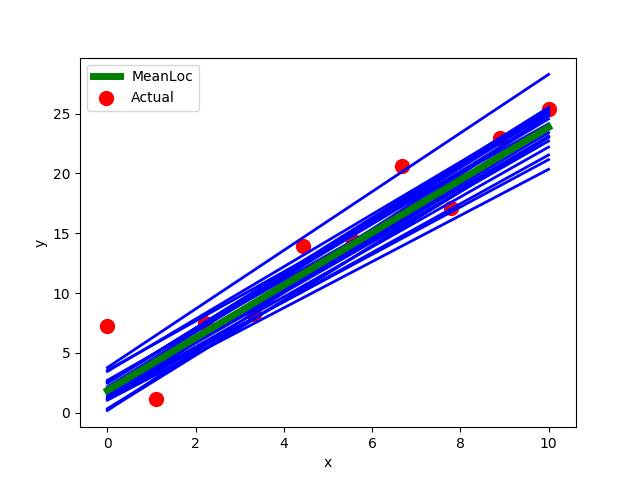
To get a better understanding of what the fitting does we can do some visualisations to make sure the model learned what we expected. In this case we just plot the raw data and the inferred regression lines from the model by sampling the posterior.

preds, loc = [], []
for i in range(20):
    borch.sample(model)
    ynew, mu = forward(model, x)
    ynew, mu = ynew.detach().numpy(), mu.detach().numpy()
    preds.append(ynew)
    loc.append(mu)
    plt.plot(x, mu, 'blue', linewidth=2.0)
mean_pred = np.stack(preds).mean(0)
mean_loc= np.stack(loc).mean(0)
plt.plot(x, mean_loc, 'g', label='MeanLoc', linewidth=5)
plt.scatter(x, y, color='r', label='Actual', s=100)
plt.xlabel('x')
plt.ylabel('y')
plt.legend()
plt.show()

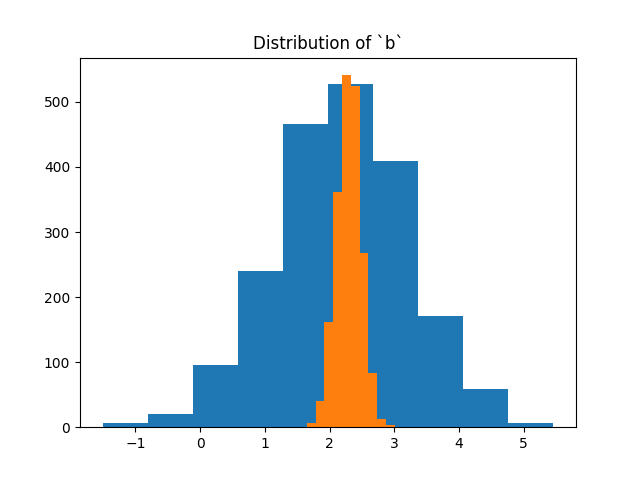
We would also like to have a look at the posterior distribution for the a and b parameter. In this case we sample 2000 samples from the a and b independently and pretend that they are from the joint posterior. We also indicate in the plot where the original model was generated from.

b = [model.posterior.b.sample().data.numpy().item() for i in range(2000)]
a = [model.posterior.a.sample().data.numpy().item() for i in range(2000)]
plt.hist(a)
plt.title('Distribution of `a`')
plt.show()
plt.hist(b)
plt.title('Distribution of `b`')
plt.show()