Introduction to Borch

Borch’s universal borch allows the creation of probabilistic models with arbitrary control flow. The core components of the borch are borch.RandomVariable and borch.nn.Module.

Lets start of with the imports:

import matplotlib

matplotlib.use("Agg")
import matplotlib.pyplot as plt
import torch

import borch
from borch import infer, distributions as dist

RandomVariable

The borch.RandomVariable merges a torch.distributions.Distribution, torch.nn.Module and a torch.tensor, it acts like a tensor and can be used just like one, but it also support methods such as .log_prob(), .entropy(), .sample(), .rsample() etc. like a torch.distributions.Distribution. It also support methods like .paramaters(), .children() etc. lake a torch.nn.Module.

A random variable is instanciated as a borch.distributions

rvar = dist.Normal(0, 1)
print(rvar)

Out:

Normal:
 loc: tensor(0.)
 scale: tensor(1.)
 posterior: Automatic()
 prior: Module()
 observed: Observed()
 tensor: tensor([])

Everytime time the random variable is called the value of the random variable gets updated with a sample from the distribution.

print(rvar())
print(rvar)
print(rvar())
print(rvar)

Out:

tensor(-1.2573)
Normal:
 loc: tensor(0.)
 scale: tensor(1.)
 posterior: Automatic()
 prior: Module()
 observed: Observed()
 tensor: tensor(-1.2573)
tensor(-0.1802)
Normal:
 loc: tensor(0.)
 scale: tensor(1.)
 posterior: Automatic()
 prior: Module()
 observed: Observed()
 tensor: tensor(-0.1802)

The tensor that represent the value of the random variable is accessible via .tensor

print(rvar.tensor)

Out:

tensor(-0.1802)

It can be used just like a normal tensor

print(rvar * 100)
print(rvar * torch.randn(10))

Out:

tensor(-18.0184)
tensor([ 0.1288, -0.1873,  0.1729, -0.0608,  0.1521, -0.0453, -0.2989,  0.1462,
         0.2152, -0.2218])

The distribution that the borch.RandomVariable is initialized with, is accessible

the method .distribution(). The method on the borch.RandomVariable differs

sightly form that of a torch.distributions.Distribution in that feeds in its own tensor as the input if no args are provided.

print(rvar.log_prob())
rvar.log_prob() == rvar.log_prob(rvar.tensor)
print(rvar.log_prob(torch.zeros(1)))

Out:

tensor(-0.9352)
tensor([-0.9189])

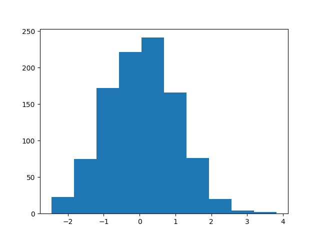
It also supports sampling(.sample()) and reparameterized sampeling(.rsample()) if available. Note that this does not update the value of the RandomVariable, only calling the RandomVariable update its value.

rvar.sample()
print(rvar)

plt.hist([rvar.sample().item() for i in range(1000)])

Out:

Normal:
 loc: tensor(0.)
 scale: tensor(1.)
 posterior: Automatic()
 prior: Module()
 observed: Observed()
 tensor: tensor(-0.1802)

(array([ 23.,  75., 172., 221., 241., 166.,  76.,  20.,   4.,   2.]), array([-2.46279907, -1.8340745 , -1.20534992, -0.57662535,  0.05209923,
        0.6808238 ,  1.30954838,  1.93827295,  2.56699753,  3.1957221 ,
        3.82444668]), <a list of 10 Patch objects>)

Module

The borch.nn.Module is an object that supports attaching and book keeping of borch.RandomVariable’s. It also got a posterior that specifies how the approximating distributions will look. It is the recommended practice to write models in two ways, either the same object oriented design as one does with torch.nn Modules.

class Model(borch.Module):
    def __init__(self):
        module.weight1 = dist.Gamma(1, 1 / 2)
        module.weight2 = dist.Normal(loc=1, scale=2)
        module.weight3 = dist.Normal(loc=1, scale=2)

    def forward(module):
        mu = module.weight1 + module.weight2 + module.weight3
        module.obs = dist.Normal(mu, 1)
        return mu

Or as functions that have a borch.nn.Module as a first argument.

def forward(module):
    module.weight1 = dist.Gamma(1, 1 / 2)
    module.weight2 = dist.Normal(loc=1, scale=2)
    module.weight3 = dist.Normal(loc=1, scale=2)
    mu = module.weight1 + module.weight2 + module.weight3
    module.obs = dist.Normal(mu, 1)
    return mu

Depending on what type of model the different syntax will be more suited then the other. Worth noting is that placing the instantiation of random variables in the __init__ method will result in less overhead then creating them for every call.

By feeding in a borch.nn.Module to the model function, the weights will be added to the borch.nn.Module object in place. The method borch.pq_to_infer(model) converts the RandomVariables that are attached to the Model object into a dict with lists, that contains p_dist, q_dist and value that can be used in the infer package.

In order to access all the parameters that we want to optimize, we run trough the model once before creating the optimizer.

module = borch.Module()
borch.sample(module) # this will sample all `RandomVariable`s in the network
forward(module)
optimizer = torch.optim.Adam(module.parameters())

Fitting a model using the infer package looks like this:

for ii in range(10):
    optimizer.zero_grad()
    borch.sample(module)
    forward(module)
    loss = infer.vi_loss(**borch.pq_to_infer(module))
    loss.backward()
    optimizer.step()

Then the fitted borch.nn.Module object can be used to generate samples. Simply by using it in the model function i.e.

for _ in range(5):
    print(forward(module))

Out:

tensor(3.8654, grad_fn=<AddBackward0>)
tensor(6.0917, grad_fn=<AddBackward0>)
tensor(-2.1938, grad_fn=<AddBackward0>)
tensor(2.3772, grad_fn=<AddBackward0>)
tensor(2.5030, grad_fn=<AddBackward0>)

Condition

For convince it would be better to specify what to condition(observe) on after the model is created and also allowing one to switch what to condition on. this can be done with

module.observe(weight2=torch.zeros(1), obs=torch.ones(1))

It will continue to condition on the values until others are provided, one can stop all conditioning by specifying

module.observe(None)

Exercises

1. Create three RandomVariable’s one with a discrete distribution, a continuous distribution that is unconstrained and a continuous distribution that has a positive support. Test the different methods on them like:

   • .samlpe()

   • .rsamlpe()

   • .log_prob()

   • .entropy()